Using Directed Acyclic Graphs (DAGs) in R for Causal Inference

Introduction

Perhaps in fulfilment of the well-known phrase “A picture is worth a thousand words”, scientists often use visual diagrams to communicate their reasoning and findings to both a wider audience and their academic peers. This practice is also prevalent in the field of causal inference, which involves determining whether a relationship between two or more variables is causal or merely associative. Because of the problem of confounding factors, selection bias, and other sources of bias associated with observational information that social scientists use, the task of finding causal relation of interest is very hard task. This is were causal diagrams comes into play.

Causal diagrams, originally developed in the fields of computer science and artificial intelligence, have over time been adopted across various social science disciplines (Cunningham 2021). These diagrams are commonly referred to as Directed Acyclic Graphs (DAGs) and they provide a systematic way to represent and reason about causal relationships.

DAGs are simply qualitative visual representations of causal relationships between one or more variables. One might ask what is the importance of using DAGs. They serve several important purposes:

1. Clarifying Assumptions: DAGs explicitly illustrate the causal reasoning that researchers assume based on their domain knowledge. This qualitative representation relies on the researcher’s prior understanding, including theoretical frameworks, anecdotal observations, and intuition about the causal relationships relevant to their topic of interest (Hernán and Robins 2010; Cunningham 2021).

2. Enhancing Focus: DAGs not only help readers of empirical research understand the researcher’s reasoning but also assist the researcher in organizing complex information. By providing a clear visual structure, DAGs enable researchers to focus on their narrative and avoid errors in causal inference (Morgan and Winship 2014).

Basics of causal graphs

In causal inference, most causal graphs are built upon at least one of three fundamental structures: chains, forks, and colliders. Understanding these basic DAG structures is crucial, especially when deciding which variables to control (adjust) in an analysis. While different fields may use varying terminology, these structures are universally recognized as the fundamental building blocks of causal DAGs. Table 1 summarizes these foundational elements.

Table 1: Table 1: Basic building blocks of causal DAGs

	Synonym	Notation	Easy way to remember (reference: Z)
Chain	mediator	X\(\rightarrow\)Z\(\rightarrow\)Y	one arrow in one out
Fork	common cuase	X\(\leftarrow\)Z\(\rightarrow\)Y	two arrows pointing away
Collider	immortality, inverted fork	Z\(\rightarrow\)Z\(\leftarrow\)Y	two arrows are pointing into it

Ploting Basics of causal graphs

To plot causal DAGs in R we need two packages:

• dagitty package which is used to create, edit and analyse causal graphs. It is a available both as a browser-based environment (https://dagitty.net/) and as R package. Eventhough, this tool is available both as browser-based tool, in this post we are using its R-package daggity, and

• ggdagis a build on top of dagity package and makes, DAG objects drawn on dagitty easier to work with it (tidying, ploting) .

In the following code chunk, I loaded the two packages which is already installed in my PC. Note that you need to install first if not using install.packages("ggdag") and install.packages("dagitty").

library(ggdag)
library(dagitty)

The process of creating DAG in R is two fold:

• first you create a DAG object using dagify() function in dagitty package

• second you plot that object (the one you created in the first step) with ggdag package.

Chain DAGs

chain <- dagify(
  y~x,
  y~z,
  z~x
)

ggdag(chain) +
  theme_dag()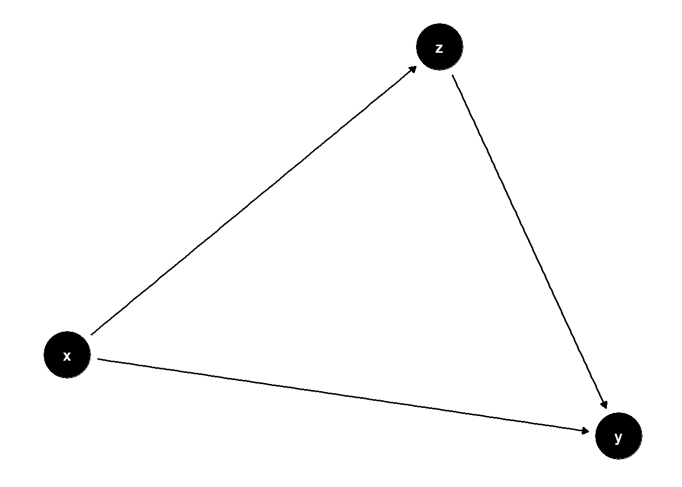

Fork

fork <- dagify(
  y~x,
  x~z,
  y~z)

ggdag(fork) +
  theme_dag()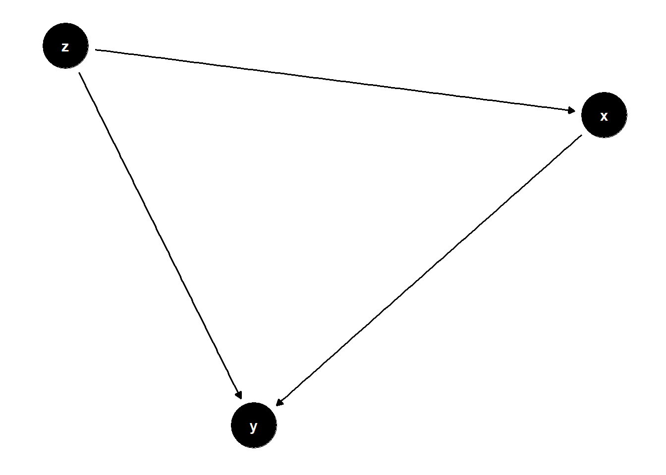

# ?dagify()

Collider

collider <- dagify(
  y~x,
  z~x,
  z~y
)
ggdag(collider)+
  theme_dag()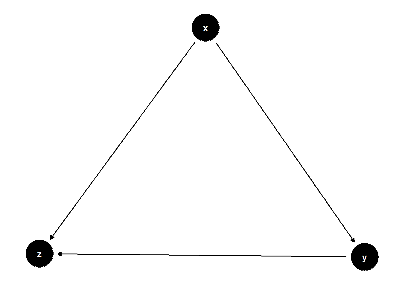

Layout:

ggdag()’s default is to randomly position nodes (variables) in random position layout every time you run/render it. If you would like to plot one fixed layout you have to either specify the coordinates of the nodes using coord argument inside the dagify() as shown in the following examples.

Chain:

chain <- dagify(
  y~x,
  y~z,
  z~x,
  coords = list(
    x = c(x = 1, z = 2, y = 3),
    y = c(x = 0, z = 1, y = 0))
)

ggdag(chain)+ 
  theme_dag()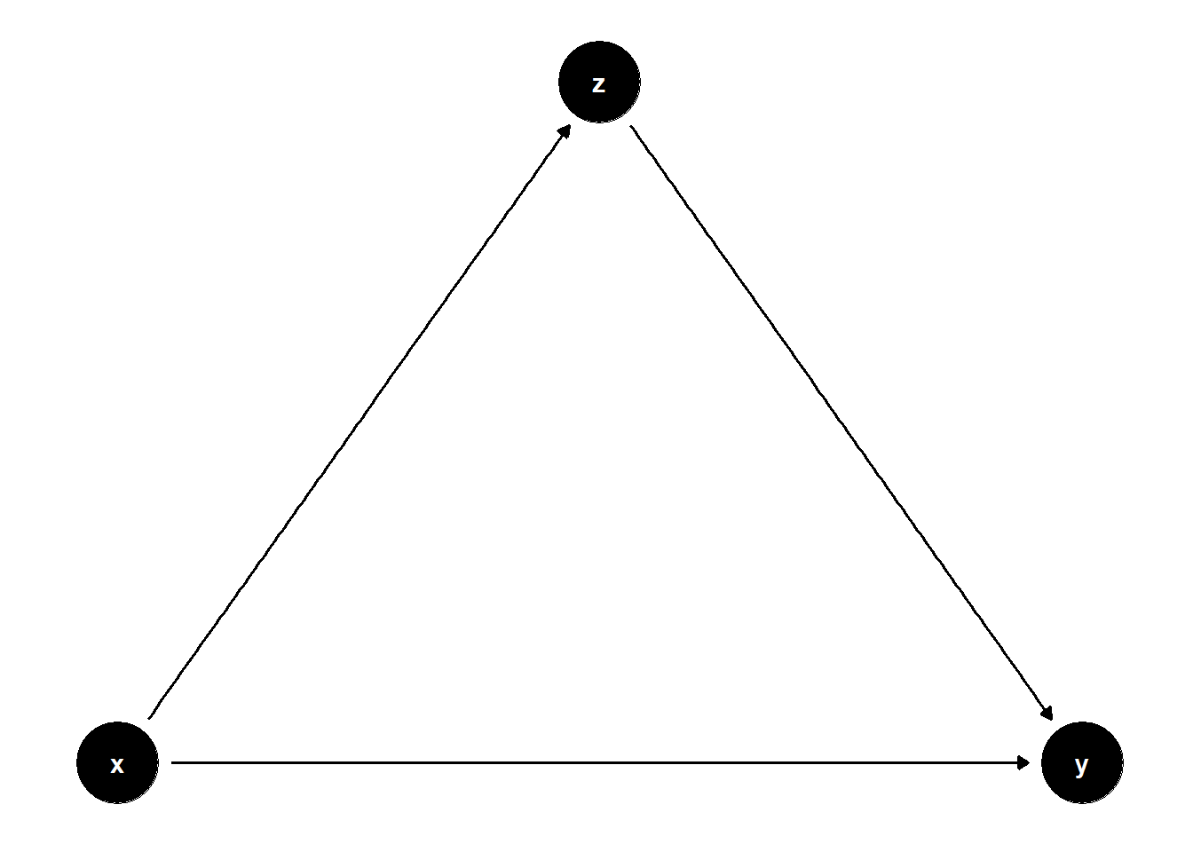

Fork:

fork <- dagify(
  y~x,
  x~z,
  y~z,
  coords = list(
    x = c(x = 1, z = 2, y = 3),
    y = c(x = 0, z = 1, y = 0))
  )

ggdag(fork) +
  theme_dag()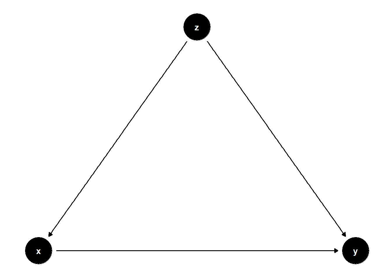

Collider:

collider <- dagify(
  y~x,
  z~x,
  z~y,
  coords = list(
    x = c(x = 1, z = 2, y = 3),
    y = c(x = 0, z = 1, y = 0))
)
ggdag(collider)+
  theme_dag()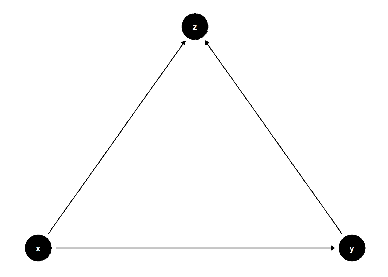

References

Cunningham, Scott. 2021. Causal Inference: The Mixtape. Yale university press.

Hernán, Miguel A, and James M Robins. 2010. “Causal Inference.” CRC Boca Raton, FL.

Morgan, Stephen L., and Christopher Winship. 2014. Counterfactuals and Causal Inference: Methods and Principles for Social Research. 2nd ed. Cambridge University Press. https://doi.org/10.1017/CBO9781107587991.